
Electromagnetic Fields Simulator: Electric, Magnetic and Light Waves
A free electromagnetism simulator: place charges and see field lines, equipotentials and Gauss's law, add current-carrying wires and check Ampere's law, turn bar magnets and see their flux lines and magnetic isopotentials, steer a charged particle through electric and magnetic fields, watch Maxwell's equations make waves reflect, refract and diffract, and explore a 3D electromagnetic plane wave.
Place charges and see the electric field they make: field lines leave positive charges and end on negative ones, equipotentials are the lines of equal voltage. Drag a charge to move it. Hover anywhere to read the field and the voltage. Draw a Gauss sphere to check Gauss's law by adding up the field on its surface.
Tip: click a charge (or sensor) to select it, then press Backspace or Delete to remove it. Drag to move it. Tape measure: drag from point to point. Voltmeter: click twice to put down the two probes (it shows red minus black voltage); drag a probe to move it.
Long straight wires that run straight through the picture: ⊙ carries current out of the screen, ⊗ into it. Each makes a magnetic field that circles round it. Add wires, drag them, and use the Ampère loop to check Ampère's law. Parallel currents attract, opposite ones repel (the arrow on the selected wire).
Bar magnets and the two families of lines around them. Flux lines (the usual “magnetic field lines”) show which way B points; they leave the N end, curve round and go back in at the S end, and carry on inside the magnet from S to N, so every line is a closed loop. Isopotentials are lines of equal magnetic scalar potential ψ, like the contour lines on a map; outside the magnet they cross the flux lines at right angles. Drag a magnet to move it, grab its round handle (or use the mouse wheel over it) to turn it.
All magnets
Tip: click a magnet to select it (the sliders then change only that one; click empty space to change all of them). R / Shift+R turns the selected magnet, Backspace or Delete removes it. The handle snaps to 5°; hold Shift while turning for any angle. Compasses: drag them around, their red end points the way B does.
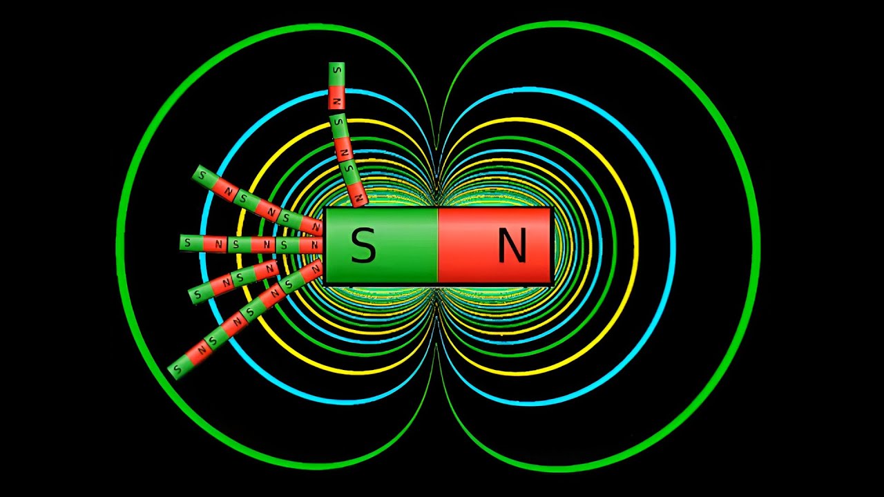 Video · MES PhysicsMagnetic Isopotentials Explain the Faraday Paradox, Stern-Gerlach Experiment, and Atomic Orbitals
Further exploration
Watch the video above, and see all of the MES Physics videos.
Lori Gardi (FractalWoman) and Michael Snyder discuss magnetic isopotentials: why the lines of equal potential, not only the flux lines, are worth drawing and measuring. Lori's channel: FractalWoman on YouTube, including her playlist On Magnetic Isopotentials.
PlayMagnet, free apps by Michael Snyder for placing magnets and seeing their isopotentials and field lines:
A charged particle in a uniform magnetic field B (pointing out of the screen, dots) and electric field E. The magnetic force bends it into circles, an electric field across it makes the circles drift sideways. Try the examples: the cyclotron, the E×B drift, the velocity selector and the mass spectrometer.
Maxwell's equations solved live on a grid (the electric field points out of the screen: red = up, blue = down). Waves reflect from metal, slow down and bend in glass, spread through slits and ring in a cavity. Pick a scene, or paint your own materials and place sources.
What an electromagnetic wave is: electric (red) and magnetic (blue) fields that oscillate at right angles to each other and to the direction the wave travels, in step, with B = E/c. Pick a kind of wave, a polarisation, and drag to rotate the view.
The wave is shown frozen-slow: a real visible light wave oscillates 500 trillion times a second.
Electricity, magnetism and light in one place
Short link to share or type on a phone: mes.fm/emf
Four equations describe all of classical electromagnetism. Gauss's law says electric field lines start on positive charge and end on negative charge. Gauss's law for magnetism says magnetic field lines never start or end: they close in loops. Faraday's law says a changing magnetic field makes an electric field, and Ampère–Maxwell says currents and changing electric fields make a magnetic field. Together they predict waves that travel at 299,792,458 m/s: light.
What each tab shows
- Electric charges. Coulomb's law adds up the field of every charge. The field lines are drawn by following the field direction from the positive charges; the closer together they are, the stronger the field. Equipotentials cross field lines at right angles. The Gauss surface adds up E·A over a sphere around the charges with numerical integration and compares it with Q/ε₀: they agree whatever the shape of the charge cloud inside, and charges outside add nothing. Switch to “long line charges” to see the 2D version, where the field falls as 1/r and the surface is a circle.
- Currents. Each straight wire makes a field μ₀I/(2πr) circling round it. The field lines are drawn as contours of the vector potential, which is exactly what field lines are. Ampère's law says the loop integral of B equals μ₀ times the current inside; the loop shows it. Try the solenoid (the field inside is uniform, outside it nearly cancels) and the coaxial cable (no field outside at all). The force between two wires is how the ampere is defined: 1 A in each, 1 m apart, makes 2×10⁻⁷ N per metre.
- Magnets. Permanent bar magnets, each a uniformly magnetised block. The field is worked out two exact ways that agree: as magnetic “charge” sheets on the two pole faces (which gives the scalar potential ψ and its isopotentials) and as the equivalent currents on the long sides (whose vector potential gives the closed flux lines, with equal flux between neighbouring lines). Turn the magnets, bring poles together, build a horseshoe or a Halbach array, and drop compasses into the field. It has its own page too: Magnetic Isopotentials.
- Charged particle. The Lorentz force makes a charge in a magnetic field go in a circle of radius r = mv/(qB) with a period 2πm/(qB) that does not depend on its speed: that is how a cyclotron works. Add an electric field across it and the circles drift sideways at E/B whatever the charge or mass. Where v = E/B the forces cancel: a velocity selector. Different masses make different circles: a mass spectrometer. At high speed the relativistic mass makes the circles bigger (switch Mechanics between Newtonian and relativistic to compare).
- Waves. A two-dimensional finite-difference time-domain (FDTD, Yee) solution of Maxwell's equations with the electric field out of the screen. Glass slows the wave to c/n and bends it (Snell's law); a metal surface forces the field to zero so the wave reflects with a sign flip; a lossy absorber turns the wave into heat; the box with metal walls is a resonant cavity that only rings at certain frequencies; two slits make an interference pattern.
- Plane wave. The textbook picture of an electromagnetic wave in three dimensions, for any wavelength from radio waves to gamma rays, with linear, circular and elliptical polarisation. The numbers (frequency, field strength, intensity, photon energy) are exact for the settings.
Accuracy and limits
The electrostatic and magnetostatic fields are exact formulas (checked against Gauss's law, Ampère's law and E = −∇V in the tests). Particle paths use the Boris integrator, which conserves the energy of a particle in a magnetic field to rounding error, with a relativistic option. The wave solver is second-order accurate: waves with fewer than about 10 cells per wavelength travel a few per cent too slowly, and the absorbing edges reflect about 1% (see the tests). It is a 2D, single-polarisation model, so it does not show magnetic-field direction or 3D effects such as Brewster's angle. Everything runs on your device and nothing is uploaded.
Light in a Medium · Michelson–Morley · Photoelectric Effect · More MES tools